
flowchart TB
    rct("Randomised controlled trial")
Moving beyond the mythical average individual
Epidemiology as driver of personalised care
Prelude
The “Average Man”?

The “Average Man”?
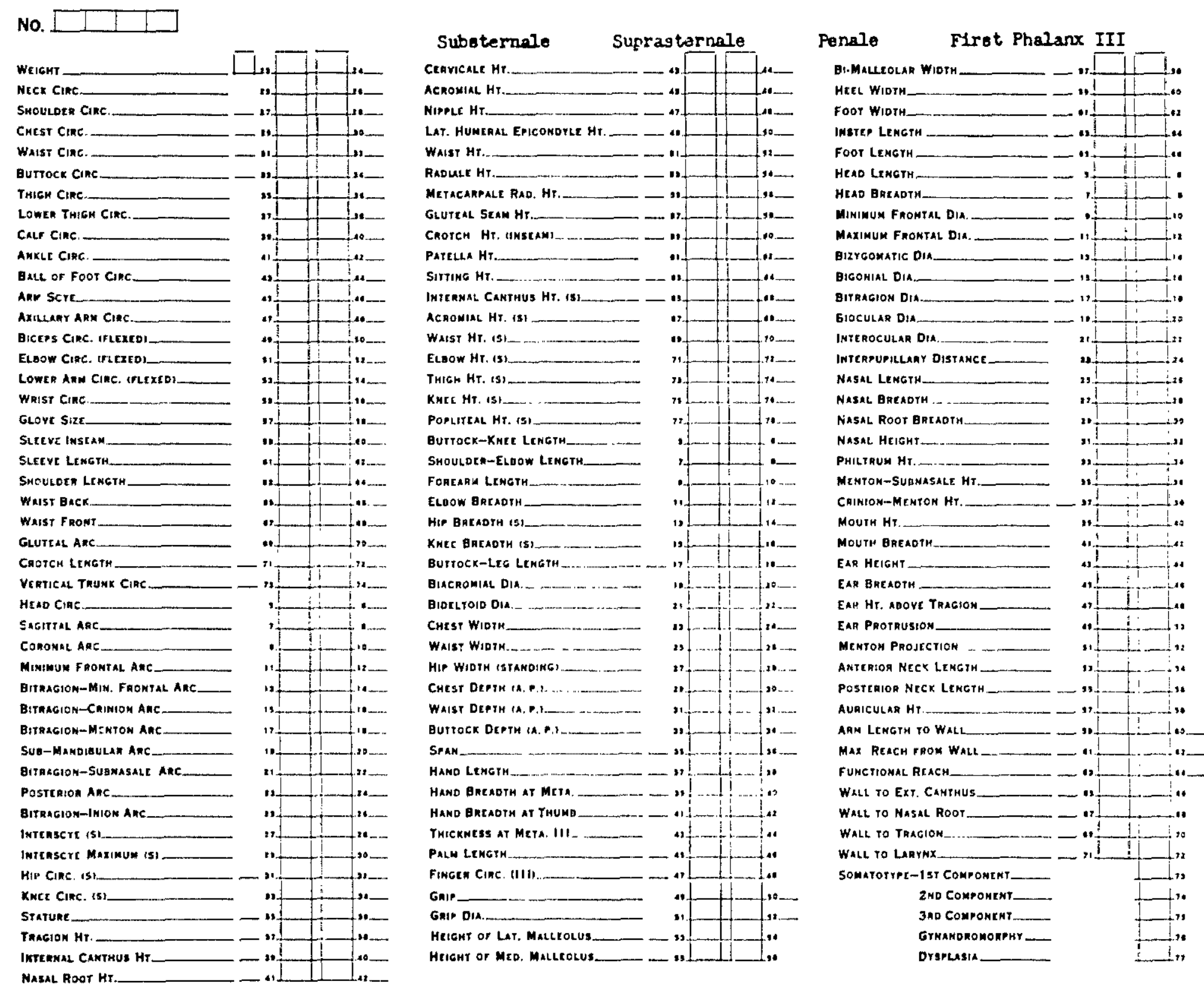
The “Average Man”?

The “Average Man”?
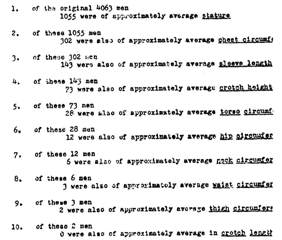
Academia’s mythical average individual
Causal aim:
- What is the effect of intervention \(A=1\) compared to intervention \(A=0\) on outcome \(Y^a\)?
Academia’s mythical average individual
Causal aim:
- What is the effect of intervention \(A=1\) compared to intervention \(A=0\) on outcome \(Y^a\)?
flowchart TB
    rct("Randomised controlled trial") --> ma["Main analysis"]
Academia’s mythical average individual
Causal aim:
- What is the effect of intervention \(A=1\) compared to intervention \(A=0\) on outcome \(Y^a\)?
flowchart TB
    rct("Randomised controlled trial") --> ma["Main analysis"]
    ma --> ate(["Average treatment effect (ATE)"])
Estimands: ATE
Average treatment effect: \[\mathbb{E}[Y^{a=1}] - \mathbb{E}[Y^{a=0}]\]
Useful for:
- Policy makers
RCTs are powered to estimate the ATE.
Academia’s mythical average individual
Causal aim:
- What is the effect of intervention \(A=1\) compared to intervention \(A=0\) on outcome \(Y^a\)?
flowchart TB
    rct("Randomised controlled trial") --> ma["Main analysis"]
    ma --> ate(["Average treatment effect (ATE)"])
Academia’s mythical average individual
Causal aim:
- What is the effect of intervention \(A=1\) compared to intervention \(A=0\) on outcome \(Y^a\)?
flowchart TB
    rct("Randomised controlled trial") --> ma["Main analysis"]
    ma --> ate(["Average treatment effect (ATE)"])
    ate --> pop("Population")
Academia’s mythical average individual
Causal aim:
- What is the effect of intervention \(A=1\) compared to intervention \(A=0\) on outcome \(Y^a\)?
flowchart TB
    rct("Randomised controlled trial") --> ma["Main analysis"]
    ma --> ate(["Average treatment effect (ATE)"])
    ate --> pop("Population")
    rct --> sa["Subgroup analysis"]
Academia’s mythical average individual
Causal aim:
- What is the effect of intervention \(A=1\) compared to intervention \(A=0\) on outcome \(Y^a\)?
flowchart TB
    rct("Randomised controlled trial") --> ma["Main analysis"]
    ma --> ate(["Average treatment effect (ATE)"])
    ate --> pop("Population")
    rct --> sa["Subgroup analysis"]
    sa --> cate(["Conditional average <br> treatment effect (CATE)"])
Estimands: CATE
Conditional average treatment effect: \[\mathbb{E}[Y^{a=1}|X] - \mathbb{E}[Y^{a=0}|X]\]
Useful for:
- Policy makers
- Healthcare providers
RCTs are rarely powered to estimate a CATE.
Estimands: CATE

Estimands: CATE
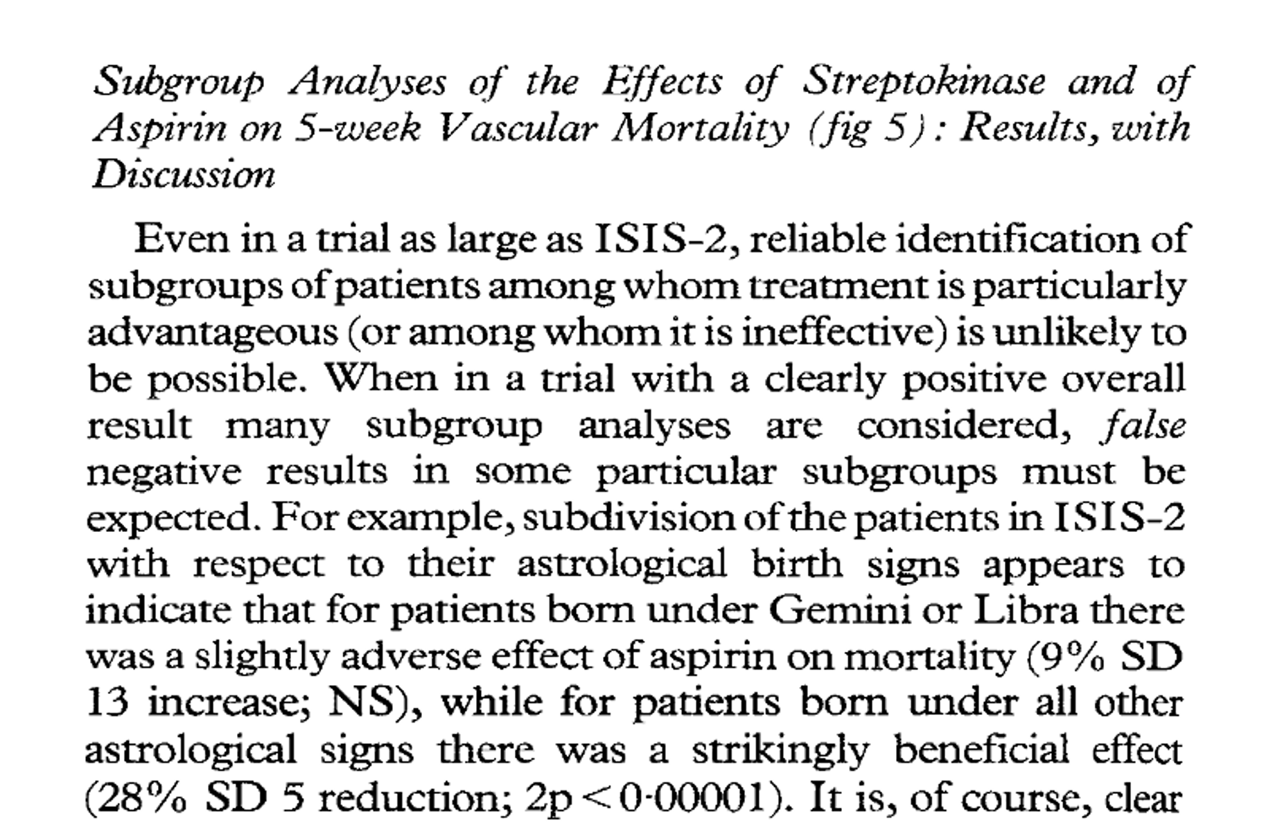
Estimands: CATE

Estimands: CATE
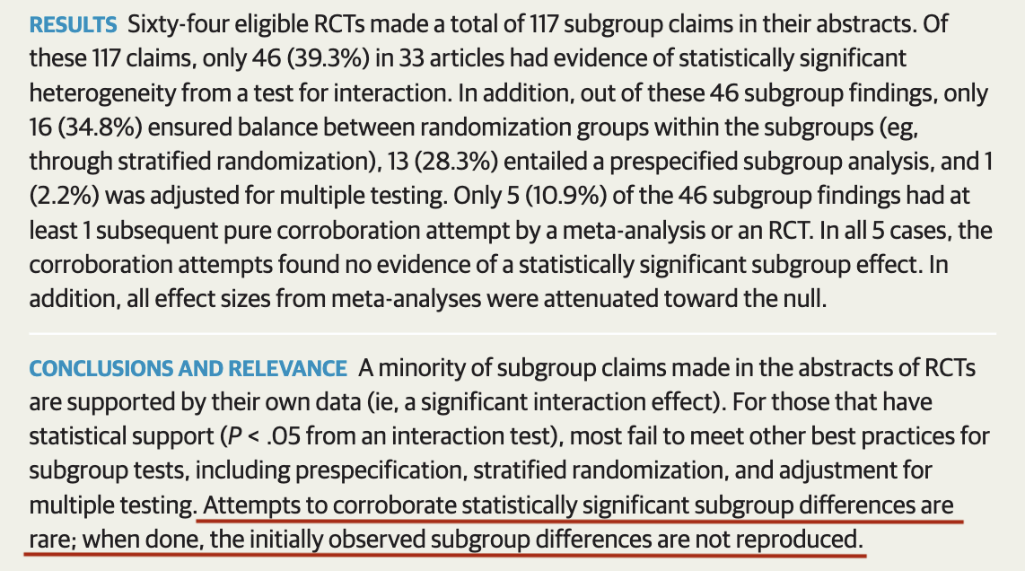
Academia’s mythical average individual
Causal aim:
- What is the effect of intervention \(A=1\) compared to intervention \(A=0\) on outcome \(Y^a\)?
flowchart TB
    rct("Randomised controlled trial") --> ma["Main analysis"]
    ma --> ate(["Average treatment effect (ATE)"])
    ate --> pop("Population")
    rct --> sa["Subgroup analysis"]
    sa --> cate(["Conditional average <br> treatment effect (CATE)"])
Academia’s mythical average individual
Causal aim:
- What is the effect of intervention \(A=1\) compared to intervention \(A=0\) on outcome \(Y^a\)?
flowchart TB
    rct("Randomised controlled trial") --> ma["Main analysis"]
    ma --> ate(["Average treatment effect (ATE)"])
    ate --> pop("Population")
    rct --> sa["Subgroup analysis"]
    sa --> cate(["Conditional average <br> treatment effect (CATE)"])
    cate --> subpop("Subgroups in population")
Academia’s mythical average individual
Causal aim:
- What is the effect of intervention \(A=1\) compared to intervention \(A=0\) on outcome \(Y^a\)?
flowchart TB
    rct("Randomised controlled trial") --> ma["Main analysis"]
    ma --> ate(["Average treatment effect (ATE)"])
    ate --> pop("Population")
    rct --> sa["Subgroup analysis"]
    sa --> cate(["Conditional average <br> treatment effect (CATE)"])
    cate --> subpop("Subgroups in population")
    rct --> path["Risk/effect modelling"]
Academia’s mythical average individual
Causal aim:
- What is the effect of intervention \(A=1\) compared to intervention \(A=0\) on outcome \(Y^a\)?
flowchart TB
    rct("Randomised controlled trial") --> ma["Main analysis"]
    ma --> ate(["Average treatment effect (ATE)"])
    ate --> pop("Population")
    rct --> sa["Subgroup analysis"]
    sa --> cate(["Conditional average <br> treatment effect (CATE)"])
    cate --> subpop("Subgroups in population")
    rct --> path["Risk/effect modelling"]
    path --> ite(["Individualised treatment <br> effect (ITE)"])
Estimands: ITE
Individualised treatment effect:
(really just a CATE) \[\mathbb{E}[Y^{a=1}|X_1,X_2...X_p] - \mathbb{E}[Y^{a=0}|X_1,X_2...X_p]\]
Useful for:
- Healthcare providers
RCTs are not powered to estimate an ITE
Academia’s mythical average individual
Causal aim:
- What is the effect of intervention \(A=1\) compared to intervention \(A=0\) on outcome \(Y^a\)?
flowchart TB
    rct("Randomised controlled trial <br> (RCT)") --> ma["Main analysis"]
    ma --> ate(["Average treatment effect (ATE)"])
    ate --> pop("Population")
    rct --> sa["Subgroup analysis"]
    sa --> cate(["Conditional average <br> treatment effect (CATE)"])
    cate --> subpop("Subgroups in population")
    rct --> path["Risk/effect modelling"]
    path --> ite(["Individualised treatment <br> effect (ITE)"])
Academia’s mythical average individual
Causal aim:
- What is the effect of intervention \(A=1\) compared to intervention \(A=0\) on outcome \(Y^a\)?
flowchart TB
    rct("Randomised controlled trial <br> (RCT)") --> ma["Main analysis"]
    ma --> ate(["Average treatment effect (ATE)"])
    ate --> pop("Population")
    rct --> sa["Subgroup analysis"]
    sa --> cate(["Conditional average <br> treatment effect (CATE)"])
    cate --> subpop("Subgroups in population")
    rct --> path["Risk/effect modelling"]
    path --> ite(["Individualised treatment <br> effect (ITE)"])
    ite --> ind("Individual people")
Academia’s mythical average individual
Causal aim:
- What is the effect of intervention \(A=1\) compared to intervention \(A=0\) on outcome \(Y^a\)?
flowchart TB
    rct("Randomised controlled trial <br> (RCT)") --> ma["Main analysis"]
    ma --> ate(["Average treatment effect (ATE)"])
    ate --> pop("Population")
    rct --> sa["Subgroup analysis"]
    sa --> cate(["Conditional average <br> treatment effect (CATE)"])
    cate --> subpop("Subgroups in population")
    rct --> path["Risk/effect modelling"]
    path --> ite(["Individualised treatment <br> effect (ITE)"])
    ite --> ind("Individual people")

%% Custom style for node CATE and ITE
style cate fill:#F9A03F,stroke:#C36F09
style ite fill:#E79E9C,stroke:#6F1D1B
Academia’s mythical average individual
Causal aim:
- What is the effect of intervention \(A=1\) compared to intervention \(A=0\) on outcome \(Y^a\)?
flowchart TB
    rct("Pooled RCTs/ <br> Observational study") --> ma["Main analysis"]
    ma --> ate(["Average treatment effect (ATE)"])
    ate --> pop("Population")
    rct --> sa["Subgroup analysis"]
    sa --> cate(["Conditional average <br> treatment effect (CATE)"])
    cate --> subpop("Subgroups in population")
    rct --> path["Risk/effect modelling"]
    path --> ite(["Individualised treatment <br> effect (ITE)"])
    ite --> ind("Individual people")
Treatment effect heterogeneity
- The CATE/ITE can differ for specific subgroups/individuals
- This is of interest if they differ in magnitude or direction
- The presence of such differences is called treatment effect heterogeneity / heterogeneity in treatment effects (HTE)
- Clinically relevant HTE occurs when the differences cross a clinically relevant threshold
- Clinically relevant HTe is generally measured on the absolute scale
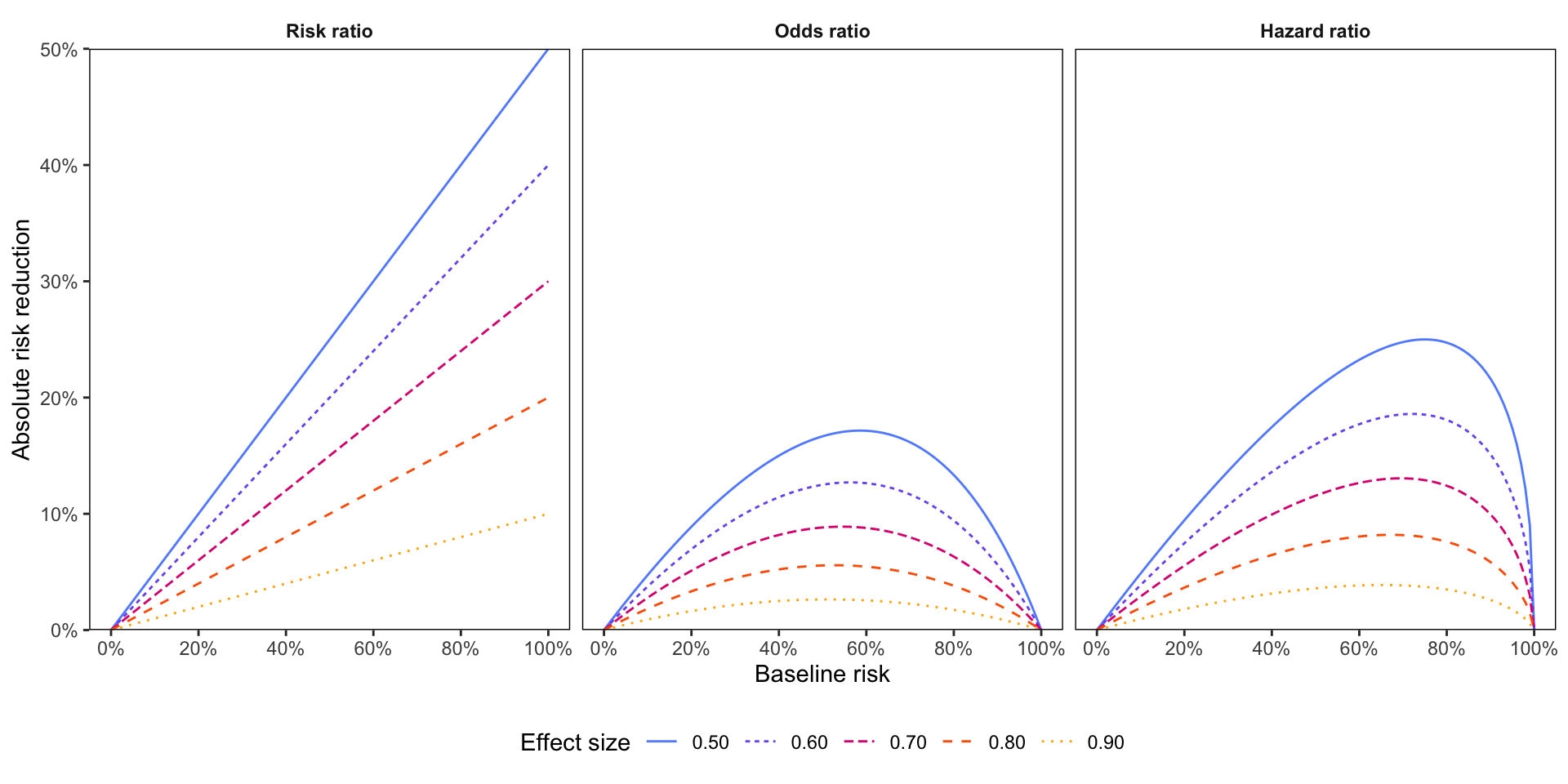
Treatment effect heterogeneity
We should note the scale of HTE: relative homogeneity may still give absolute heterogeneity:
Treatment effect heterogeneity
- One way to investigate and estimate HTE is through prediction modelling
- Corresponding methodology is summarised in the Predictive Approaches to Treatment effect Heterogeneity (PATH) statement

The PATH statement
(and more)
PATH approaches
- Risk modelling
Incorporate individual baseline risk (\(E\)) into analyses - Effect modelling
Directly estimate individualised treatment effect
Risk modelling
General concept: Incorporate individual baseline risk (\(E\)) into analyses
- Method 1: add treatment-risk interaction to outcome model (\(\mathbb{E}[Y^{a,e}]\))
This gives an indication of the statistical presence of HTE on the relative scale - Method 2: perform analyses in risk-based subgroups (\(\mathbb{E}[Y^a|E]\))
This gives the CATE based on strata of predicted baseline risk
Important
When performing subgroup analyses, ensure that exchangeability holds
Risk modelling: Baseline risk
How to estimate the individual baseline risk?
Their baseline risk is their conditional probability of the outcome (\(Pr(Y|X_1,X_2,...X_p)\)) and can be estimated using an:
- internal model (developed within the study data)
- external model (developed in external data)
Important
Internal models should be developed in the population not receiving the treatment of interest
Risk modelling: Baseline risk
External models are available in abundance:

Risk modelling: Baseline risk
Regardless of the model used:
- validate it in your own data
Is your identification/CATE valid in your population? - validate it in your target population
Can you transfer your estimates to your target population?
Effect modelling
General concept: Directly estimate individualised treatment effect
In case exchangeability holds:
- Each individual contributes to estimation in their factually assigned treatment arm
- Given exchangeability, we may use differently assigned individuals to consider an individual’s counterfactual situation if they were assigned to the other treatment arm
- We can model the causal contrast between individuals with contrasting treatment arms, conditional on a sufficient set of individual predictors \(\textbf{X}\) (\(\textbf{X} = X_1,X_2...X_p\))
- Given \(\textbf{X}\), this causal contrast reflects the individual benefit (a.k.a. the individualised treatment effect)
- Ideally, benefit is estimated on the absolute scale, e.g. the absolute risk difference (ARD)
Effect modelling
Several techniques for effect modelling,exist:
- S-learner
- T-learner
- X-learner
- DR-learner: double-robust estimator (treatment + outcome model)
- R-learner: model residuals after removing variance through covariates
- Causal forest: random data splits to maximise treatment effect differences
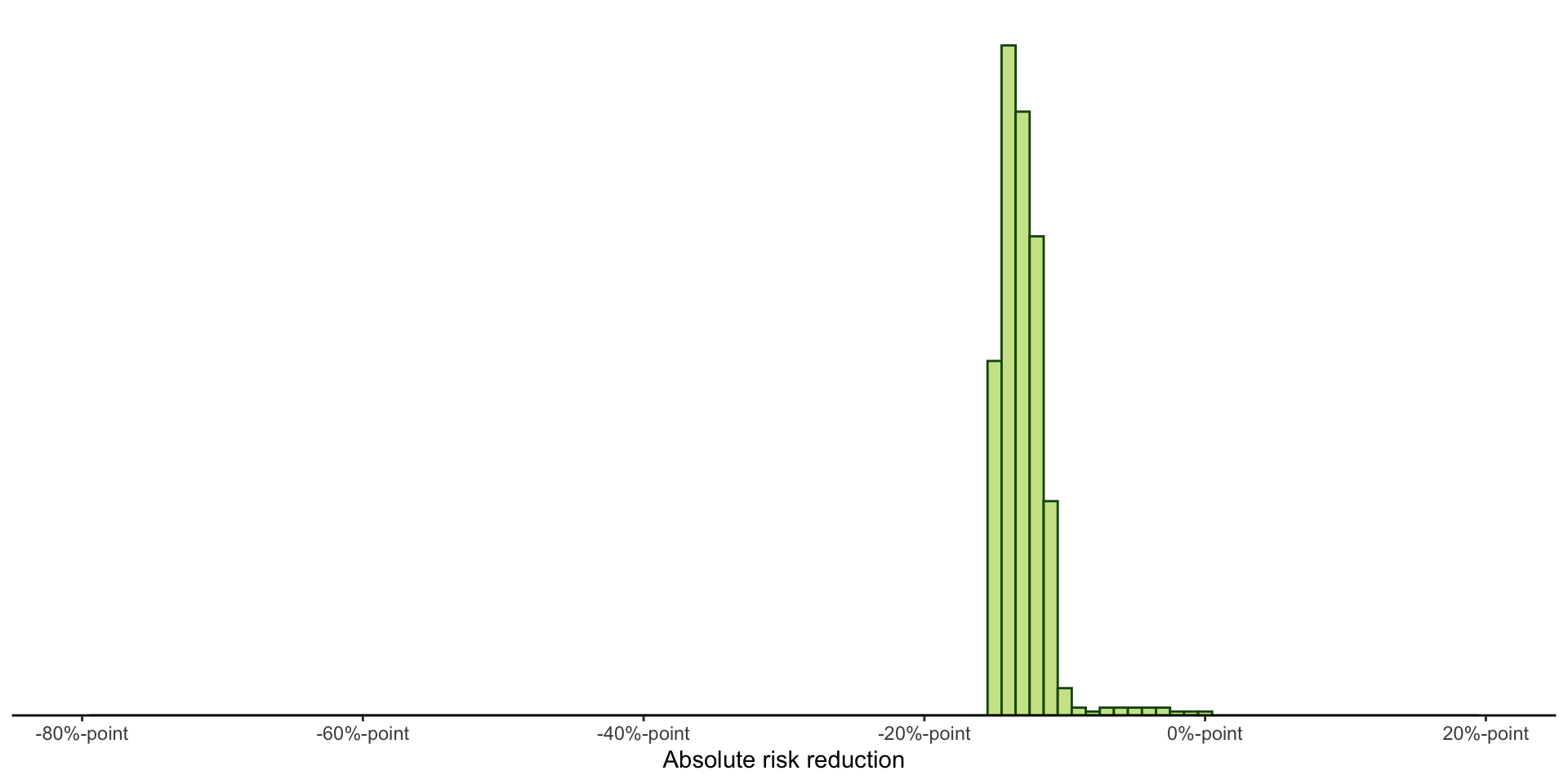
S-learners
S-learners are the simplest method, as they rely on only a single model:
- We aim to estimate the \(ARD\), as estimand for individual benefit
- We express this as \(ARD = AR_{A=1} - AR_{A=0}\), where \(AR_{A=1} = \mathbb{E}[Y=1|A=1,\textbf{X}]\) and \(AR_{A=0} = \mathbb{E}[Y=1|A=0,\textbf{X}]\)
- An S-learner means that we fit a single (S) model for both \(AR_{A=1}\) and \(AR_{A=0}\)
- Thus, we fit the model \(\hat{\mu}(x)\) as \(M(Y \sim A + \textbf{X})\)
- We then calculate benefit as \(ARD = \hat{\mu}(x,A = 1) - \hat{\mu}(x,A = 0)\)
Note
\(M\) can be any model architecture we desire
S-learners
An example using data from one of the first succesful trials of adjuvant chemotherapy in colon cancer (Levamisole + 5-FU vs. placebo) 1
# A tibble: 619 × 11
      id   trt female   age obstruct perfor adhere nodes differ  time death
   <dbl> <dbl>  <dbl> <dbl>    <dbl>  <dbl>  <dbl> <dbl> <fct>  <dbl> <dbl>
 1     1     1      0    43        0      0      0     5 2       1521     1
 2     2     1      0    63        0      0      0     1 2       3087     0
 3     3     0      1    71        0      0      1     7 2        963     1
 4     4     1      1    66        1      0      0     6 2        293     1
 5     5     0      0    69        0      0      0    22 2        659     1
 6     6     1      1    57        0      0      0     9 2       1767     1
 7     8     0      0    54        0      0      0     1 2       3192     0
 8    10     1      1    68        0      0      0     1 2       3308     0
 9    12     1      0    52        0      0      0     2 3       3309     0
10    13     0      0    64        0      0      0     1 2       2085     1
# ℹ 609 more rowsS-learners
We also need a small function to get the outcome risk:
ar <- function(.data,         # Data with predictors
               trt_status,    # Hypothetical treatment status
               fit            # Model fit
){
    # Get linear predictor with hypothetical new data
    lp <- predict(fit,
                  type = "lp",
                  newdata = mutate(.data, trt = trt_status))

    # Get AR
    ar <- 1 - (exp(-last(basehaz(fit))[["hazard"]]) ^ exp(lp))

    # Return output
    return(ar)
}
S-learners
S-learners
T-learners
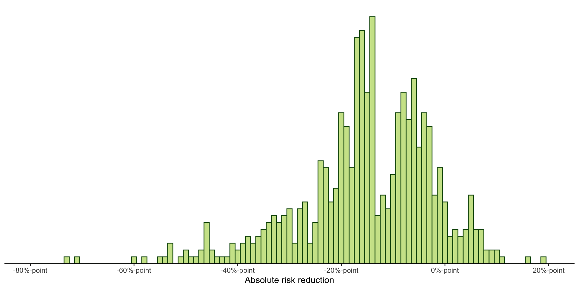
T-learners instead use a single model per treatment arm. In our example, that would be two (T) models.
- A T-learner means that we fit separate models for \(AR_{A=1}\) and \(AR_{A=0}\)
- Thus, we fit the models
\(\hat{\mu}_1(x)\) as \(M(Y^1 \sim \textbf{X}^1)\);
\(\hat{\mu}_0(x)\) as \(M(Y^0 \sim \textbf{X}^0)\) - We then calculate benefit as \(ARD = \hat{\mu}_1(x) - \hat{\mu}_0(x)\)
T-learners
T-learners
# Subset data
dat_a1 <- filter(dat, trt == 1)   # Treated population
dat_a0 <- filter(dat, trt == 0)   # Untreated population
# Fit treated model
fit_tlearner_a1 <- coxph(Surv(time, death) ~ age + female + obstruct + perfor + adhere + nodes + differ,
data = dat_a1)
# Fit untreated model
fit_tlearner_a0 <- coxph(Surv(time, death) ~ age + female + obstruct + perfor + adhere + nodes + differ,
data = dat_a0)T-learners
# Subset data
dat_a1 <- filter(dat, trt == 1)   # Treated population
dat_a0 <- filter(dat, trt == 0)   # Untreated population

# Fit treated model
fit_tlearner_a1 <- coxph(Surv(time, death) ~ age + female + obstruct + perfor + adhere + nodes + differ,
                         data = dat_a1)

# Fit untreated model
fit_tlearner_a0 <- coxph(Surv(time, death) ~ age + female + obstruct + perfor + adhere + nodes + differ,
                         data = dat_a0)
# Estimate ARD
vec_ard <- ar(dat, NULL, fit_tlearner_a1) - ar(dat, NULL, fit_tlearner_a0)T-learners
X-learners
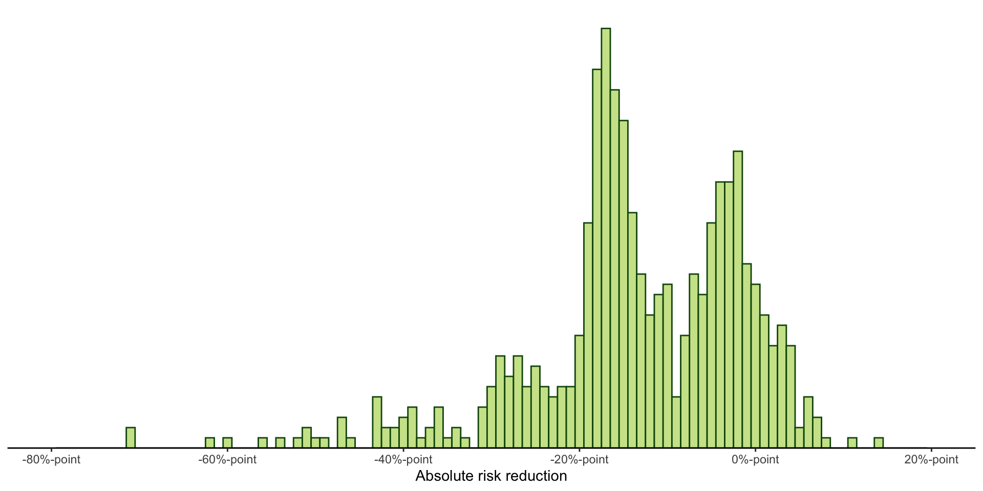
An X-learner similarly fits two models, like the T-learner, but uses them in a cross-over manner (hence X):
- We again fit separate models for \(AR_{A=1}\) and \(AR_{A=0}\):
\(\hat{\mu}_1(x)\) as \(M(Y^1 \sim \textbf{X}^1)\);
\(\hat{\mu}_0(x)\) as \(M(Y^0 \sim \textbf{X}^0)\) - We then use the treated model to counterfactually predict what the control group would have experienced under treatment and vice versa:
\(\hat{\mu}_1(\textbf{X}^0)\);
\(\hat{\mu}_0(\textbf{X}^1)\) - These counterfactual predictions allow us to impute the treatment effects by subtracting them from observed outcomes:
\(D^1 = Y^1 - \hat{\mu}_1(\textbf{X}^0)\);
\(D^0 = \hat{\mu}_0(\textbf{X}^1) - Y^0\)
X-learners
- We now fit two new models for the imputed treatment effects:
\(\hat{\tau_1}(x)\) as \(M(D^1 \sim \textbf{X}^1)\);
\(\hat{\tau_0}(x)\) as \(M(D^0 \sim \textbf{X}^0)\) - Last, we can combine the estimates from these models:
\(ARD = g(x) * \hat{\tau_0}(x) + (1 - g(x)) * \hat{\tau_1}(x))\) - Here, \(g(x)\) is a weighting factor, which generally equals the propensity score \(PS = \mathbb{E}[A|\textbf{X}]\), estimated as \(M(A \sim \textbf{X})\)
X-learners
X-learners
# Subset data
dat_a1 <- filter(dat, trt == 1)   # Treated population
dat_a0 <- filter(dat, trt == 0)   # Untreated population
# Fit treated model
fit_xlearner_a1 <- coxph(Surv(time, death) ~ age + female + obstruct + perfor + adhere + nodes + differ,
data = dat_a1)
# Fit untreated model
fit_xlearner_a0 <- coxph(Surv(time, death) ~ age + female + obstruct + perfor + adhere + nodes + differ,
data = dat_a0)X-learners
# Subset data
dat_a1 <- filter(dat, trt == 1)   # Treated population
dat_a0 <- filter(dat, trt == 0)   # Untreated population

# Fit treated model
fit_xlearner_a1 <- coxph(Surv(time, death) ~ age + female + obstruct + perfor + adhere + nodes + differ,
                         data = dat_a1)

# Fit untreated model
fit_xlearner_a0 <- coxph(Surv(time, death) ~ age + female + obstruct + perfor + adhere + nodes + differ,
                         data = dat_a0)
# Get counterfactual predictions
vec_cf_pred_a1 <- ar(dat_a1, NULL, fit_xlearner_a0) # Treated population
vec_cf_pred_a0 <- ar(dat_a0, NULL, fit_xlearner_a1) # Untreated populationX-learners
# Subset data
dat_a1 <- filter(dat, trt == 1)   # Treated population
dat_a0 <- filter(dat, trt == 0)   # Untreated population

# Fit treated model
fit_xlearner_a1 <- coxph(Surv(time, death) ~ age + female + obstruct + perfor + adhere + nodes + differ,
                         data = dat_a1)

# Fit untreated model
fit_xlearner_a0 <- coxph(Surv(time, death) ~ age + female + obstruct + perfor + adhere + nodes + differ,
                         data = dat_a0)

# Get counterfactual predictions
vec_cf_pred_a1 <- ar(dat_a1, NULL, fit_xlearner_a0)  # Treated population
vec_cf_pred_a0 <- ar(dat_a0, NULL, fit_xlearner_a1)  # Untreated population
# Impute treatment effects
dat_a1[["d"]] <- dat_a1[["death"]] - vec_cf_pred_a1
dat_a0[["d"]] <- vec_cf_pred_a0 - dat_a0[["death"]]X-learners
# Subset data
dat_a1 <- filter(dat, trt == 1)   # Treated population
dat_a0 <- filter(dat, trt == 0)   # Untreated population

# Fit treated model
fit_xlearner_a1 <- coxph(Surv(time, death) ~ age + female + obstruct + perfor + adhere + nodes + differ,
                         data = dat_a1)

# Fit untreated model
fit_xlearner_a0 <- coxph(Surv(time, death) ~ age + female + obstruct + perfor + adhere + nodes + differ,
                         data = dat_a0)

# Get counterfactual predictions
vec_cf_pred_a1 <- ar(dat_a1, NULL, fit_xlearner_a0)  # Treated population
vec_cf_pred_a0 <- ar(dat_a0, NULL, fit_xlearner_a1)  # Untreated population

# Impute treatment effects
dat_a1[["d"]] <- dat_a1[["death"]] - vec_cf_pred_a1
dat_a0[["d"]] <- vec_cf_pred_a0 - dat_a0[["death"]]
# Fit treated model on imputed treatment effect
fit_xlearner_d_a1 <- lm(d ~ age + female + obstruct + perfor + adhere + nodes + differ,
data = dat_a1)
# Fit untreated model on imputed treatment effect
fit_xlearner_d_a0 <- lm(d ~ age + female + obstruct + perfor + adhere + nodes + differ,
data = dat_a0)X-learners
# Subset data
dat_a1 <- filter(dat, trt == 1)   # Treated population
dat_a0 <- filter(dat, trt == 0)   # Untreated population

# Fit treated model
fit_xlearner_a1 <- coxph(Surv(time, death) ~ age + female + obstruct + perfor + adhere + nodes + differ,
                         data = dat_a1)

# Fit untreated model
fit_xlearner_a0 <- coxph(Surv(time, death) ~ age + female + obstruct + perfor + adhere + nodes + differ,
                         data = dat_a0)

# Get counterfactual predictions
vec_cf_pred_a1 <- ar(dat_a1, NULL, fit_xlearner_a0)  # Treated population
vec_cf_pred_a0 <- ar(dat_a0, NULL, fit_xlearner_a1)  # Untreated population

# Impute treatment effects
dat_a1[["d"]] <- dat_a1[["death"]] - vec_cf_pred_a1
dat_a0[["d"]] <- vec_cf_pred_a0 - dat_a0[["death"]]

# Fit treated model on imputed treatment effect
fit_xlearner_d_a1 <- lm(d ~ age + female + obstruct + perfor + adhere + nodes + differ,
                        data = dat_a1)

# Fit untreated model on imputed treatment effect
fit_xlearner_d_a0 <- lm(d ~ age + female + obstruct + perfor + adhere + nodes + differ,
                        data = dat_a0)
# Estimate propensity score
dat[["ps"]] <- predict(
# Propensity score model
glm(trt ~ age + female + obstruct + perfor + adhere + nodes + differ,
data = dat,
family = binomial),
# Return PS
type = "response")X-learners
# Subset data
dat_a1 <- filter(dat, trt == 1)   # Treated population
dat_a0 <- filter(dat, trt == 0)   # Untreated population

# Fit treated model
fit_xlearner_a1 <- coxph(Surv(time, death) ~ age + female + obstruct + perfor + adhere + nodes + differ,
                         data = dat_a1)

# Fit untreated model
fit_xlearner_a0 <- coxph(Surv(time, death) ~ age + female + obstruct + perfor + adhere + nodes + differ,
                         data = dat_a0)

# Get counterfactual predictions
vec_cf_pred_a1 <- ar(dat_a1, NULL, fit_xlearner_a0)  # Treated population
vec_cf_pred_a0 <- ar(dat_a0, NULL, fit_xlearner_a1)  # Untreated population

# Impute treatment effects
dat_a1[["d"]] <- dat_a1[["death"]] - vec_cf_pred_a1
dat_a0[["d"]] <- vec_cf_pred_a0 - dat_a0[["death"]]

# Fit treated model on imputed treatment effect
fit_xlearner_d_a1 <- lm(d ~ age + female + obstruct + perfor + adhere + nodes + differ,
                        data = dat_a1)

# Fit untreated model on imputed treatment effect
fit_xlearner_d_a0 <- lm(d ~ age + female + obstruct + perfor + adhere + nodes + differ,
                        data = dat_a0)

# Estimate propensity score
dat[["ps"]] <- predict(
    # Propensity score model
    glm(trt ~ age + female + obstruct + perfor + adhere + nodes + differ,
        data = dat,
        family = binomial),
    # Return PS
    type = "response")
# Final estimate
vec_ard <-
# No treatment
dat[["ps"]] * predict(fit_xlearner_d_a0, newdata = dat) +
# Treatment
(1 - dat[["ps"]]) * predict(fit_xlearner_d_a1, newdata = dat)X-learners
Performance
Why we’re not yet done
- Our models for ITE estimates are in fact prediction models
- As such, we need to validate them, at least on:
Calibration: how well does the predicted benefit correspond with the true benefit?
Discrimination: how well can the model distinguish those with low and with high benefit? - One problem: validation is difficult because we do not know the true benefit (as we can never observe the counterfactual)
- Thus we rely on suboptimal measures that approach the true benefit for validation
Note
Despite all our best efforts to individualise estimates, model performance metrics generally reflect the average population or a coarse subgroup: a model that performs adequate on average does not reflect individual adequacy of the model
Calibration
Approach 1: Grouping
- Divide population into quantiles and compare the average predicted benefit against the average observed benefit
- For the absolute risk difference, this can be differences in the KM-estimator (or CIF) between treated and untreated
- We can also calculate calibration-in-the-large using this method
- This approach assumes exchangeability holds in the created quantiles (otherwise, the observed ARR is not valid)
- Instead of using all available information, data is reduced to quantiles
Calibration
Approach 2: Matching (calibration-for-benefit)
- Match treated and untreated individuals, either on predicted benefit or underlying individual characteristics
- Calculate pairwise observed benefit:
0 (both died or both survived); 1 (treated died, untreated survived); -1 (treated survived, untreated died) - Calculate parwise predicted benefit:
Difference in factual predictions (i.e. according to actual treatment) - Draw a calibration curve (and calculate metrics) with a smoother on predicted pairwise and observed pairwise benefit
- This approach assumes pairwise benefit is a good alternative to individual benefit estimates
- The matching procedure used has considerable influence on the results
Calibration
Simulated data (so that we know true benefit)
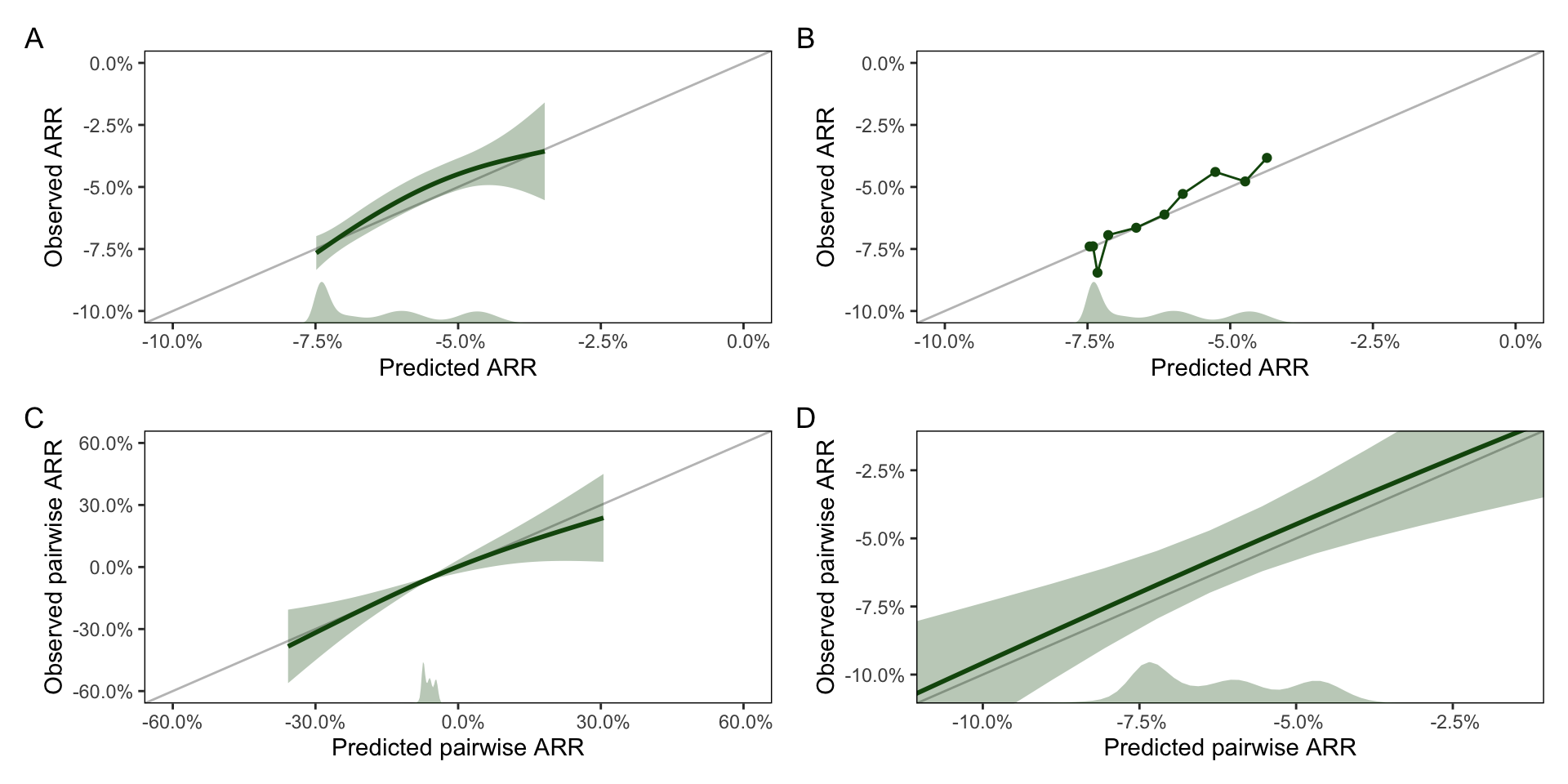
Calibration
Our S-learner
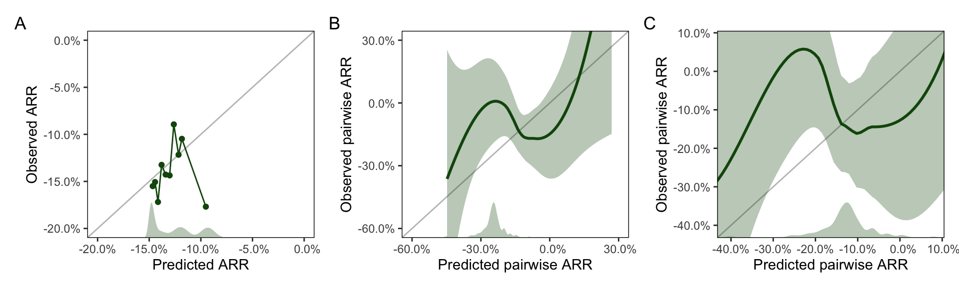
Discrimination
Approach 1: C-for-benefit
- As with calibration-for-benefit: match first
- Then, calculate pairwise benefit (observed and predicted)
- Calculate C-statistic as usual
- Still sensitive to matching procedure
- Pairwise benefit does not equal individual benefit
- C-for-benefit is improper!
Discrimination
Approach 2: Concentration of benefit (\(C_b\))
- Efficiency of a prediction model in assigning treatment, compared to random treatment assignment
- Uses random sampling of benefit
- Strong assumption: benefit is correctly calibrated;
\(C_b\) does not incorporate outcome in its calculation - Thus, we cannot interpret it with poor calibration
- Ideally 100%, or 50% if all predicted benefits have a single direction
Discrimination
For \(C_b\), we thus only need the estimated benefit:
Discrimination
Approach 3: Qini curves
- Weight your outcome (\(Y\)) by the propensity score (\(PS\)):
\(Y^* = \frac{Y(A - PS)}{PS(1 - PS)}\)
Upweight individuals who received treatment/no treatment contrary to what we expected based on the propensity score - Rank your population (of size \(n\)) from highest to lowest benefit (\(ARD\))
- Create a decision rule \(\pi\) to treat the top \(\phi\) percent:
\(\pi_\phi = \begin{cases}1, & if \hspace{0.1cm} ARD \ge top \hspace{0.11cm} \phi\%\\0, & otherwise\end{cases}\) - Calculate the gain corresponding to the proportion treated \(g(\phi)\):
\(g(\phi) = \frac{1}{n}\displaystyle\sum^n_i\pi_{\phi}Y^*\) - Iterate over all relevant proportions
Discrimination
Approach 3: Qini curves
We can also incorporate individual costs:
- Adjust individual benefit \(ARD_i\) with individual cost \(C_i\):
\(ARD^* = \frac{ARD_i}{C_i}\) - Rank your population from highest to lowest cost-adjusted benefit (\(ARD^*\))
- Create a decision rule \(\pi\) to treat the top \(\phi\) percent and calculate the gain \(g(\phi)\)
- Calculate the cost corresponding to the proportion treated \(c(\phi)\):
\(c(\phi) = \frac{1}{N_\phi}\displaystyle\sum^{N_\phi}_iC_i\) - Adjust treated proportion to account for incurred costs:
\(\phi^* = g(\phi) * c(\phi)\) - Iterate over all relevant proportions and report \(g(\phi)\) for \(\phi^*\)
Discrimination
First we define a function for the Qini curve
# Function to calculate gain per spend for Qini curve
qini <- function(benefit,                      # CATE/ITE, assuming higher = more benefit
                 trt,                          # 1 = treated, 0 = not treated (according to factual assignment)
                 outcome,                      # 1 = outcome, 0 = no outcome
                 ps,                           # Propensity score
                 cost = 1,                     # Incurred costs per individual
                 phi_low = 0,                  # Lowest proportion assessed
                 phi_high = 1,                 # Highest proportion assessed
                 output = c("curve", "table")  # Should curve be drawn or table be given
){
    # Match output
    output <- match.arg(output)

    # Create tibble for computations
    dat_qini <- tibble(id = 1:length(benefit),
                       benefit,
                       trt,
                       outcome,
                       ps,
                       cost)

    # Calculate gain for each proportion
    dat_qini_final <- bind_rows(lapply(seq(phi_low, phi_high, length.out = nrow(dat_qini)), \(x){
        # Rank data
        dat_tmp <- dat_qini %>%
            # Scale benefit by cost
            mutate(benefit = benefit / cost) %>%
            # Rank on benefit
            arrange(desc(benefit))

        # Determine treated individuals according to pi
        vec_treat_ids <- dat_tmp[1:round(quantile(1:nrow(dat_tmp), prob = x)), ][["id"]]

        # Compute weighted outcome and gain
        dat_tmp %<>%
            # Computations
            mutate(# Treatment assignment
                   treat = if_else(id %in% vec_treat_ids, 1, 0),
                   # Random treatment assignment (ATE approach)
                   treat_ate = rbinom(nrow(dat_tmp), 1, x),
                   # Weighted outcome
                   y_star = outcome * (trt - ps) / (ps * (1 - ps)),
                   # Costs are only incurred by treated individuals
                   cost = if_else(treat == 1, cost, NA),
                   # Costs for ATE approach
                   cost_ate = if_else(treat_ate == 1, cost, NA),
                   # Calculate gain
                   gain = treat * y_star,
                   # Calculate ATE gain
                   gain_ate = treat_ate * y_star)

        ## CATE approach
        # Calculate mean gain
        mean_gain <- mean(dat_tmp[["gain"]])

        # Calculate mean cost
        mean_cost <- mean(dat_tmp[["cost"]], na.rm = TRUE)

        # Adjust spend for cost if it differed per individual
        if(n_distinct(cost) > 1) spend <- x * mean_cost else spend <- x

        # Qini table for CATE
        dat_cate <- tibble(type = "cate",
                           spend = spend,
                           gain = mean_gain)

        ## ATE approach
        # Calculate mean gain
        mean_gain_ate <- mean(dat_tmp[["gain_ate"]])

        # Calculate mean cost
        mean_cost_ate <- mean(dat_tmp[["cost_ate"]], na.rm = TRUE)

        # Adjust spend for cost if it differed per individual
        if(n_distinct(cost) > 1) spend_ate <- x * mean_cost_ate else spend_ate <- x

         # Qini table for ATE
        dat_ate <- tibble(type = "ate",
                          spend = spend_ate,
                          gain = mean_gain_ate)

        # Combine tables
        dat_tab <- bind_rows(dat_cate, dat_ate)


        # Return table
        return(dat_tab)
    }))

    # Check if table is final output
    if(output == "table") return(dat_qini_final)

    # Otherwise, output plot
    else {
        # Draw plot
        p <- ggplot(filter(dat_qini_final, type == "cate"),
                    aes(x = spend,
                        y = gain)) +
            # Geometries
            geom_line(colour = "#13540c") +
            geom_smooth(mapping =
                            aes(x = filter(dat_qini_final, type == "ate")[["spend"]],
                                y = filter(dat_qini_final, type == "ate")[["gain"]]),
                        method = "lm",
                        formula = "y ~ x",
                        se = FALSE,
                        colour = "black",
                        linetype = "dashed",
                        linewidth = 0.5) +
            # Scaling
            scale_x_continuous(name = "Portion of population treated",
                               breaks = seq(0, 1, 0.2),
                               labels = paste0(seq(0, 100, 20), "%")) +
            scale_y_continuous(name = "Gain") +
            # Aesthetics
            theme_manual()

        # Return plot
        return(p)
    }
}
Discrimination
On simulated data:
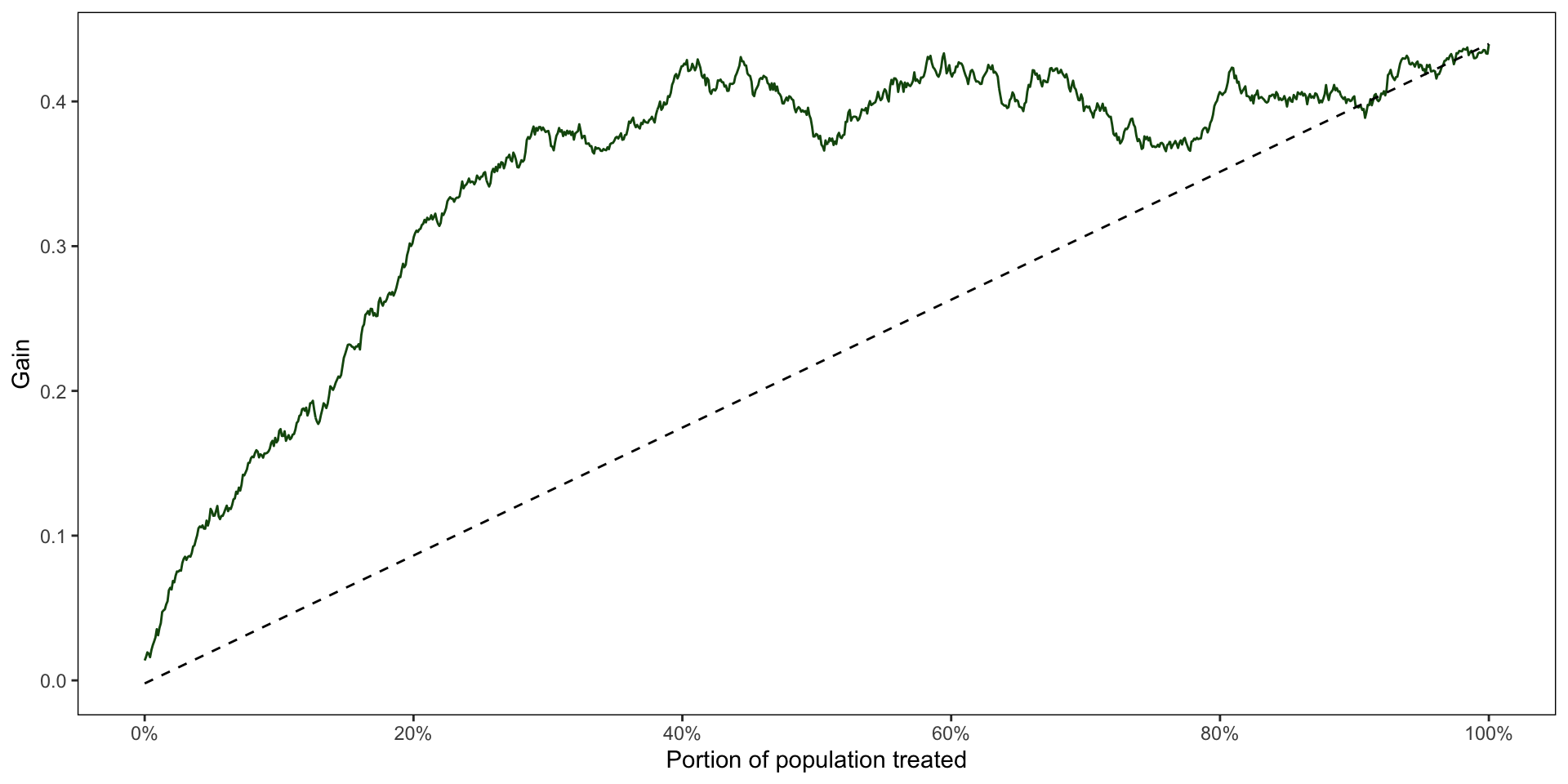
Discrimination
Our S-learner:
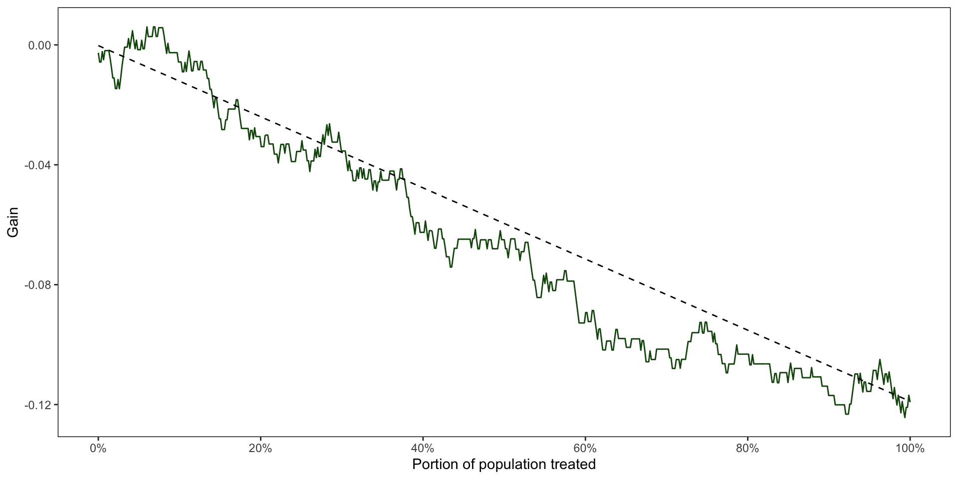
Cautionary notes
Exchangeability
Warning
- All these techniques assume exchangeability, but do not make groups exchangeable themselves.
- Randomised controlled trials are a common data source for these analyses, but rarely represent the target population
- Observational data can be used if the underlying design gives (conditional) exchangeability
(e.g. T-learner in a cloning-censoring-weighting design)
Sample size
Warning
- Randomised controlled trials are almost always powered only for their ATE, not for any specification of the ATE like a CATE or ITE
- Pooled randomised controlled trials may suffice, but this is not a guarantee
- Observational data may suffice, but larger data sources often lose granularity
- Sample size calculations rarely factor in all sources of variation and formal sample size calculations are not available for these methods
- Prediction intervals are your (computationally intensive) best friend!
Validation
Warning
- Your data source might not fully represent your target population
- Validate for both internal and external validity of estimates
- Target your validation: “external validation” means nothing without context
Clinical implementation
Warning
“A prediction model that is not used has as much clinical impact as a prediction model that was never developed” - Roemer J. Janse, 2026
We can put as much effort, data, and complex statistics into our model as we want, but if it is not used, it did not matter. After development, there is a long road to walk from validation to market approval to implementation. Do not walk that road alone: involve your stakeholders.
Thank you!
- Web: rjjanse.github.io
- Contact: r.j.janse-5@umcutrecht.nl
- Slides: rjjanse.github.io/talks
- Code: github.com/rjjanse