Creating data

Annotation

Let’s get started in R. Before we write any code, we should discuss the importance of annotation. When you are writing code it might seem clear to you what each line does, but if someone else reads your code or you look back at your code after a while, it might not seem so clear anymore. To allow others and your future-self to efficiently check, read, and re-use your code, it is important to extensively annotate your code. Let’s see some unannotated code (you don’t have to understand now what the code means):

iris %>%
    filter(Species == "setosa") %>%
    extract2("Sepal.Length") %>%
    is_greater_than(5) %>%
    table() %>%
    prop.table() %>%
    extract2(TRUE) %>%
    `*`(100) %>%
    paste0(., "%")

In this section of code, there is a lot that happens (although some R users might still get the gist of the code). Moreover, a single section of code might quickly get much longer and more complicated than the above example. Luckily, the code can added to with annotation. In R, you can annotate with ‘#’. Any text written after the ‘#’ on the same line will not be run by R and can therefore be used to annotate code. So let’s see how we can increase this code’s clarity with annotation:

# Calculate proportion of setosa observations with sepal length above 5
iris %>%
    # Keep only setosa species
    filter(Species == "setosa") %>%
    # Keep only the sepal length values
    extract2("Sepal.Length") %>%
    # Determine whether each value is greater than 5 or not
    is_greater_than(5) %>%
    # Count lengths above and below 5
    table() %>%
    # Turn counts into proportions
    prop.table() %>%
    # Keep only proportion for lengths above 5
    extract2(TRUE) %>%
    # Multiply by 100
    `*`(100) %>%
    # Add percentage sign
    paste0(., "%")

It is true that annotation increases the length of a script, but it is important to note that the quality of a script is not affected by its length, but it is by its clarity.

You can use annotation for more than just explaining what your code does. You can add information on the general purpose of a script, its author, its creation date. You can add information on why you made a certain decision or add a URL to where you found the solution to a coding problem. It is easy to annotate too little, but difficult to annotate too much.

Basic mathematic operators and running code

Now let’s (finally) see some real code! Let’s start with some basic operators:

1 + 1   # Addition
3 - 1   # Substraction
2 * 3   # Multiplication
8 / 2   # Division
8 %% 2  # Modulo

R follows the conventional order of mathematic operation.

However, these operators are useless if we do not actually run the code. To run a section of code, put your cursor in the code section (can be anywhere) and press ctrl + enter to run the code. If you want to run a specific part of the code, instead of a whole section, you can select the part you want to run and then use ctrl + enter again, to run only the selected part.

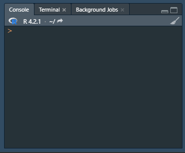
The results of the selected code can be found in the console. If the code takes some time to run, you can see it is done when a new line of the console starts with > (Figure 1 (a)).

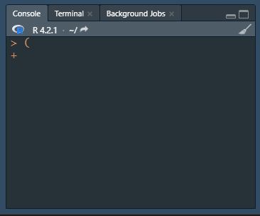
If you select a specific part of code to run, make sure to be inclusive! For instance, if you forget to select an enclosing paranthesis, the selected code will be put in the console, but it will not be run. You can see that this happened if a new line in the console starts with + (Figure 1 (b)). To cancel a waiting command, you can press esc.

If we run the example code for the basic mathematic operators, we will get the following results:

1 + 1   # Addition

[1] 2

3 - 1   # Substraction

[1] 2

2 * 3   # Multiplication

[1] 6

8 / 2   # Division

[1] 4

8 %% 2  # Modulo

[1] 0

Before each result, you can see [1]. This indicates that that specific line of code starts with the n^th result. When a single code starts printing multiple results, this can help identify what n a certain result is.

Functions

Now that we know the basic mathematic operators, we could calculate the standard deviation. For example, for the numbers 3, 8, 3, 7 and 1, we could do the following:

# Calculate the mean
(3 + 8 + 3 + 7 + 1) / 5

[1] 4.4

# Use the calculated mean to calculate the standard deviation
(((3 - 4.4) ^ 2 + (8 - 4.4) ^ 2 + (3 - 4.4) ^ 2 + (7 - 4.4) ^ 2 + (1 - 4.4) ^ 2) / (5 - 1)) ^ 0.5

[1] 2.966479

A sample’s standard deviation \(s\) is obtained by calculating:

\[\sqrt\frac{\sum{(x-\overline{x})^2}}{n-1}\]

However, with only 5 numbers, this is already a lot of effort. This is where functions come in: R has many built-in keywords that allow you to quickly perform operations and/or calculations on the data, which we call functions. A function has a generic name and is followed by opening and closing brackets. Between the brackets, we can supply so-called arguments (i.e., data and/or specifications). For example, if we wanted to calculate the standard deviation, instead of typing out all the numbers, we could just type the following:

# Calculate standard deviation
sd(c(3, 8, 3, 7, 1))

[1] 2.966479

In the standard deviation function, we use the c() function. Later we will elaborate on this, but for now it is enough to remember that c() creates a collection of data, which is more often called an object.

Be aware that R is case-sensitive: c() as a function differs from C().

Let’s see some standard functions that will be of great help to you.

Sum

sum(), as it name suggests, sums the supplied values. It has the following arguments:

...: the ellipsis indicates that any number of values can be supplied here. The sum function can take numeric values, integers, and booleans/logicals (i.e., it can sum the amount of TRUEs).
na.rm = FALSE: na.rm indicates whether any missing values should be dropped. By default, this is FALSE, meaning that the function will return NA if there is any NAs present in the data you are trying to sum. If you want to sum all valid values (thus drop all NAs), you can specify na.rm = TRUE.

See the below examples:

sum(3, 4, 5, 6)

[1] 18

sum(3, NA, 5, 6)

[1] NA

sum(3, NA, 5, 6, na.rm = TRUE)

[1] 14

In the sum() function, na.rm has the default value FALSE. This means that this argument does not have to be defined. If we would not define it, it would just use FALSE.

Mean and median

To get the mean or median from some data, you can use the mean() and median() functions. mean() has the following arguments:

x: a collection (or object) of data containing the data for which a mean should be calculated.
trim = 0: what proportion of the outskirts of the data should be trimmed (e.g., 0.05 trims 5% of data on each side). It defaults to 0.
na.rm = FALSE: whether NAs should be dropped (as in sum())

median() has the same arguments, except that it doesn’t have trim.

Here are some examples:

mean(c(3, 4, 8, 3, 0, 4, 7, 8, 3, 1, 1044))

[1] 98.63636

mean(c(3, 4, 8, 3, 0, 4, 7, 8, 3, 1, 1044), trim = 0.1)

[1] 4.555556

median(c(3, 4, 8, 3, 0, 4, 7, 8, 3, 1, 1044))

[1] 4

Notice how with the mean, we specified that 0.1 was the value for trim, but we did not specify that c(3, 4, 8, 3, 0, 4, 7, 8, 3, 1, 1044) was the value for x. This is because R inputs values for arguments in order: the first supplied value will be used for the first argument, the second supplied value will be used for the second argument, etc. However, sometimes I do not want to specify the second value, but I do want to specify the third value. In this case I can name the argument as in trim = 0.1, so that R knows the 0.1 is meant for trim.

Min and max

Now that we know how to calculate the mean and median from some data, we might also be interest in finding the lowest and highest value (for example, to detect the 1044 outlier). We can do this with min() and max(), which both take only one argument: ... as in the sum() function.

To get the minimum and maximum value from the data we just calculated the mean and median of, we could do the following:

min(3, 4, 8, 3, 0, 4, 7, 8, 3, 1, 1044)

[1] 0

max(3, 4, 8, 3, 0, 4, 7, 8, 3, 1, 1044)

[1] 1044

Summary and quintile

Now we know how to calculate the mean, median, minimum, and maximum values from some data, but what if we also want to know the 1^st and 3^rd quartile? Additionally, we do not want to use a function for each separate value. In this case, you can use summary(), which calculates the minimum, 1^st quartile, mean, median, 3^rd quartile, and maximum all at once. The summary function has multiple arguments, but only one is relevant for now:

object: the data of which you want to get a summary.

For example:

summary(c(3, 4, 8, 3, 0, 4, 7, 8, 3, 1, 1044))

   Min. 1st Qu.  Median    Mean 3rd Qu.    Max. 
   0.00    3.00    4.00   98.64    7.50 1044.00

However, maybe we are more interested in the 1^st and 99^th quantiles. In that case we could use quantile(). You can supply the following arguments to quantile():

x: a collection of data (or object) of which you want to calculate quantiles.
probs = seq(0, 1, 0.25): the probabilities (or quantiles) you want to calculate. It defaults to seq(0, 1, 0.25), which just means a sequence from 0 to 1 with increments of 0.25.
na.rm = FALSE: whether NAs should be dropped.
names = TRUE: whether the output should show the name (or specified quantile).

So we could do:

quantile(c(3, 4, 8, 3, 0, 4, 7, 8, 3, 1, 1044), 
         probs = c(0.01, 0.99))

   1%   99% 
  0.1 940.4

quantile(c(3, 4, 8, 3, 0, 4, 7, 8, 3, 1, 1044), 
         probs = c(0.01, 0.99), names = FALSE)

[1]   0.1 940.4

Table

We have now seen some functions that we can use to get some descriptives about continuous data. However, sometimes we just want to count the amount of different observations. For this we can use table(). Some of the relevant arguments for the table function are the following:

...: the variables to be supplied to table, as we saw in earlier functions.
useNA = c("no", "ifany", "always"): should NAs be tabulated (conditional on if any are present) or not. The c("no", "ifany", "always"), means that useNA takes any of the three following values: "no", "ifany", or "always".

For example:

table(c(TRUE, FALSE, FALSE, TRUE, TRUE, TRUE, TRUE, FALSE, NA))


FALSE  TRUE 
    3     5

table(c(TRUE, FALSE, FALSE, TRUE, TRUE, TRUE, TRUE, FALSE, NA), 
      useNA = "ifany")


FALSE  TRUE  <NA> 
    3     5     1

table(c(TRUE, FALSE, FALSE, TRUE, TRUE, TRUE, TRUE, FALSE), 
      useNA = "always")


FALSE  TRUE  <NA> 
    3     5     0

You can also use table() to create a cross-table:

table(c(FALSE, TRUE, FALSE, FALSE, TRUE, TRUE, TRUE, TRUE, FALSE), 
      c(TRUE, TRUE, FALSE, FALSE, TRUE, FALSE, FALSE, FALSE, FALSE))

       
        FALSE TRUE
  FALSE     3    1
  TRUE      3    2

For the cross-tabulation, values are compered based on their order in the data you supply (e.g., the first value, FALSE in the first set is compared to the first value, TRUE, in the second set.)

We now went through some arguments for commonly used functions together, but it is good that you know what arguments a function takes and where you can find this. If you want to know more about any function, for example for sum(), you can open the documentation by running ?sum. In the help panel on the lower right in RStudio, you will find the documentation with the function, its default values, elaboration on the arguments it takes, details, and examples. You can also click on a function and press F1 to open the help panel.

Storing values

We have now seen how we can calculate some values using basic mathematic operators and functions. However, just typing out our data can become quite tiresome, so preferably I would store them in a variable. In R, things that store data are often called subjects. Let’s look at some different ways we can store data.

Single value

We can assign a single value by using the <- operator (which has the easy keyboard shortcut alt + - in RStudio). To then see the object, we can simply run it. For example:

x <- sum(4, 9)
x

[1] 13

x <- 4 + 5
x

[1] 9

Note that we defined the object x twice. When defining an object that already exists, the old object is overridden.

To assign a value to an object, you can also use = instead of <-. However, this is often unclear and may be confused with defining arguments in functions. It is therefore strongly recommended to only assign objects using <-.

Vectors

When we want to assign multiple values to a single variable, we can create a vector. There are two simple ways to create a vector. First, we can use the c function (c()), that we saw before when discussing functions. c() creates a simple collection of any type of value. We call this collection a vector.

x <- c(4, 6, 9, 3, 2)
x

[1] 4 6 9 3 2

# Using a vector in the sum function
sum(x)

[1] 24

You can also create a vector of sequential integers by using ::

x <- 5:17
x

 [1]  5  6  7  8  9 10 11 12 13 14 15 16 17

Additionally, you can create any sequence using the seq() function which takes the arguments from, to, and by, meaning respectively the start, finish, and increments of the sequence.

x <- seq(5, 7, 0.5)
x

[1] 5.0 5.5 6.0 6.5 7.0

We could also multiply two vectors with each other (given they have the same length) or a vector with a single value:

x <- 1:5
y <- 5:1

x * y

[1] 5 8 9 8 5

x * 2

[1]  2  4  6  8 10

Lastly, you could create a named vector (i.e., each value has a name):

x <- c("Obs1" = 42, "Obs2" = 28, "Obs3" = 91)
x

Obs1 Obs2 Obs3 
  42   28   91

Lists

A list is also a collection of data, but it can store much more than just values, such as vectors, and whole data sets:

x <- list(head(iris, 3), head(mtcars, 3))
x

[[1]]
  Sepal.Length Sepal.Width Petal.Length Petal.Width Species
1          5.1         3.5          1.4         0.2  setosa
2          4.9         3.0          1.4         0.2  setosa
3          4.7         3.2          1.3         0.2  setosa

[[2]]
               mpg cyl disp  hp drat    wt  qsec vs am gear carb
Mazda RX4     21.0   6  160 110 3.90 2.620 16.46  0  1    4    4
Mazda RX4 Wag 21.0   6  160 110 3.90 2.875 17.02  0  1    4    4
Datsun 710    22.8   4  108  93 3.85 2.320 18.61  1  1    4    1

However, you cannot immediately apply mathematic operators on a list or use a list in data. If we have a list with data (for example different objects), we first have to unlist:

x <- list(4, 2)
unlist(x) * 2

[1] 8 4

When you create a model, they are always stored in lists too, with many information alongside the results. We will come across this later in the tutorial.

Matrices

If we want data with more than one dimension (i.e., columns and rows), we could create a matrix with the matrix function:

x <- matrix(c(31, 3, 18, 7, 84, 20), nrow = 3, ncol = 2)
x

     [,1] [,2]
[1,]   31    7
[2,]    3   84
[3,]   18   20

We can also supply a single value that fills the entire matrix:

x <- matrix("Hello, World!", nrow = 5, ncol = 3)
x

     [,1]            [,2]            [,3]           
[1,] "Hello, World!" "Hello, World!" "Hello, World!"
[2,] "Hello, World!" "Hello, World!" "Hello, World!"
[3,] "Hello, World!" "Hello, World!" "Hello, World!"
[4,] "Hello, World!" "Hello, World!" "Hello, World!"
[5,] "Hello, World!" "Hello, World!" "Hello, World!"

Matrices are useful because they have multiple dimensions, which allows us to store different variables of the same person in multiple columns along the same row.

Data frames

Matrices give us a flexible way to store data with rows and columns, but miss some flexibility when it comes to manipulating the data and performing calculations, loading it into functions, etc. In this case, data frames offer a good solution. Data frames look exactly matrices, but are much easier to manipulate and use for analyses. Data frames are likely what will compose most of the data you use in R.

We can create a data frame with the data.frame() function:

x <- data.frame(id = 1:5,
                value1 = c(5, 2, 0, 2, 4),
                value2 = c(9.4, 8.3, 2.8, 5.6, 2.7))
x

  id value1 value2
1  1      5    9.4
2  2      2    8.3
3  3      0    2.8
4  4      2    5.6
5  5      4    2.7

When working with data frames, there are some useful functions you can use:

To determine how many rows and columns a data frame (or matrix) has, you can use nrow() and ncol().
To change the row and column names, you can use rownames() and colnames(). To see how these functions work, you can access the examples in their documentation with ?rownames and ?colnames.
To change a data frame to a matrix or a matrix to a data frame, you can use as.matrix() and as.data.frame().

The global environment

We have seen some ways to create and store data now. However, where can we find back what we have created? This is where the global environment comes in. Whenever you create an object in your code, that object will be stored in the global environment, which is just a general storage space. A great benefit that RStudio gives us is being able to see the global environment and whatever is stored in there, and to get a quick indication of what kind of data is stored.

Before we see the global environment, let’s first clean it with the following code:

rm(list = ls())

With the rm() function, we can remove objects from our global environment, and here we specify that the list of variables to be removed (list =), is the whole global environment (ls()). It is useful to remove objects you do not need to keep your global environment clean. Not only does it help in available working memory, it is also good to work in an organized (global) environment.

Now let’s create some new data to showcase the global environment in RStudio:

# Load pre-existing data frame
data <- iris

# Create vector
vector <- 1:13

# Create single value
val <- 42

# Create vector of strings
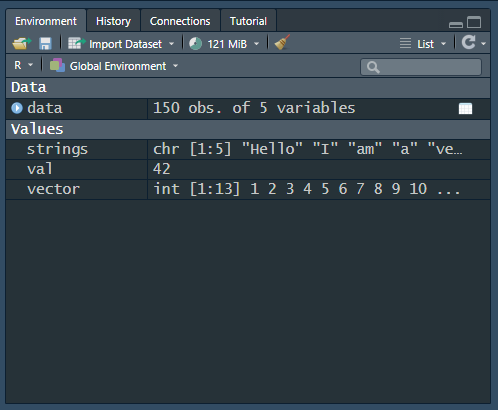
strings <- c("Hello", "I", "am", "a", "vector")

Now let’s look at our global environment. If you remember, the upper right window of the RStudio interface shows the global environment. With the data we just created, it will look like Figure 2 (a) (the colours might differ depending on your theme).

From the global environment, we can learn a few things:

The current memory usage is 121 MiB, in the upper middle of the image.
We have one structured data object, data. This data object has 150 observations (rows) of 5 variables (columns).
strings is a character (chr) with 5 values ([1:5). We then see the first values.
val is a single value, 42.
vector is an integener (int) with 13 values ([1:13]`) and we can see the first values.

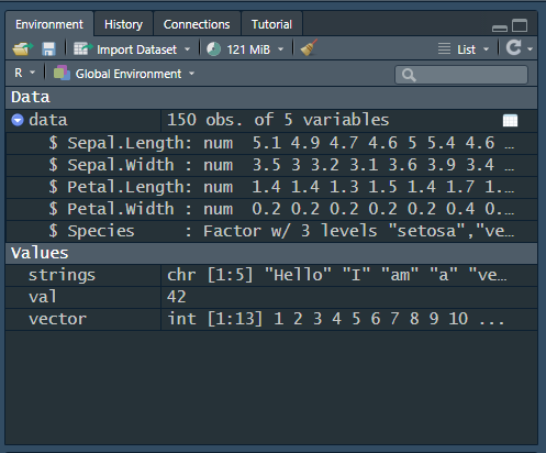
This already gives us quite some information, but we can also get some more information on the structured data. If you press the small blue button with an arrow, next to data, you will see that it opens, as in Figure 2 (b). This let’s us learn the following information about data:

We can see each of the columns of data. The first four are numerical (num).
The fifth column, Species, is a factor (i.e., categorical) with three levels (of which the first one is “setosa”).

global environment — (a) Global environment

global environment with opened data — (a) Global environment

Dealing with warnings and errors

We have now gone through the basics of creating and storing data. However, sometimes, we supply a wrong value to a function or mess up a parenthesis somewhere. This can give either warnings or errors. In both cases, it is important to realize what is happening. Warnings are messages printed in the console that try to tell us that something might be wrong in the data or not suited, or that the data was manipulated in the function to make sure the function could work. For example, if I try to change a character string to numeric with as.numeric(), I will get the warning: Warning message: NAs introduced by coercion, but the function still completed.

Sometimes, warnings are expected or not a problem. In that case, you can put the whole code inside the function supressWarnings(), to silence the warning. It is however always of paramount importance that you annotate what the warning was and why it can be suppressed.

Sometimes, you might get an error instead of a warning. This means that the function could not continue to run and you have to fix the error before being able to run the function.

Not all errors are as clear and you can not always figure out by yourself what is going wrong. Luckily, we have the internet! You can easily google the error and add ‘R’ at the end to find other people who encountered the same or similar problems and find solutions. If you can find nothing, you could always ask on coding forums, such as stackoverflow. When you ask a solution to a coding question, always supply your question with a reproducible example, so that a responder can run the code themselves and see where it goes wrong.

Exercises

1. Create and store numbers

Create a vector of the integers 5, 6, 7, 8, 9, and 10 and store it in an object called vec.

Answer

# Answer 1: using c()
vec <- c(5, 6, 7, 8, 9, 10)

# Answer 2: using the `:` operator
vec <- 5:10

# Answer 3: using seq()
vev <- seq(5, 10, 1)

2. Calculate quantiles

Calculate the 2.5^th and 97.5^th percentile of the object vec.

Answer

quantile(vec, probs = c(0.025, 0.975))

 2.5% 97.5% 
5.125 9.875

3. Create a matrix

Using the data in vec, create a matrix with two columns and three rows.

Answer

matrix(vec, nrow = 3, ncol = 2)

     [,1] [,2]
[1,]    5    8
[2,]    6    9
[3,]    7   10

4. Getting help

Open the documentation for rm().

Answer

?rm

5. Cleaning up

Now use rm() to remove vec again.

Answer

rm(vec)

Next topic

Now that we went through the basics of creating and storing data, we can start talking about accessing and manipulating data.

Next: Using data